[분류 문제]
• 신규고객에게 신용카드를 발급하려고 하는데 어느 등급으로 해야 할까?
• 어떤 부류의 고객이 신용등급이 높을까?
• 어떤 구매자가 반품할 확률이 높을까?
• 새로 관찰한 식물은 어느 종에 속할까?
디시전 트리 분석
- 데이터를 여러 그룹으로 분류하여 변수간 나타나는 의사결정규칙을 트리구조로 분류하는 방법
디시전 트리를 만드는 알고리즘
- 엔트로피와 정보획득이론을 기반으로 하는 머신러닝 분야의 ID3, C4.5, C5.0 알고리즘
- 통계학에 기반으로 둔 CART와 CHAID
C5.0
- 엔트로피(entropy)와 정보이득(information gain) 개념에 기반을 둠
- 초기 목표변수의 데이터들이 혼재되어 있으면 무질서도, 엔트로피가 큼.
- 입력변수들의 데이터들을 분류하는 과정에서 목표변수의 데이터가 그룹화되면 엔트로피가 낮아지고 정보이득 발생
- 정보이득을 가장 크게하는 입력변수를 우선적으로 의사결정나무의 root로 분류


예시

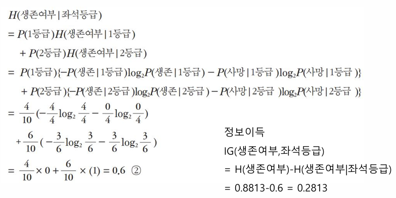
목표변수(생존여부)의 엔트로피가 0보다 크기 때문에 다음 단계로 진행.

좌석등급으로 나누었을때 정보이득
성별로 나누었을때 정보이득
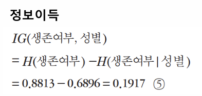
좌석등급으로 나눴을때 정보이득이 더 크다. 즉 좌석등급을 성별보다 더 높은 노드로.
종료 여부
엔트로피가 0이거나 입력변수가 남아 있지 않을때까지 계속 진행.
실습

1단계: 패키지 설정
from sklearn import tree
from sklearn.metrics import confusion_matrix, accuracy_score
from matplotlib import pyplot as plt
2단계: 데이터 준비
# 학습용 데이터
X_train = [[1, 1], [1, 1], [1, 1], [1, 0], [2, 1], [2, 1], [2, 1], [2, 1], [2, 0], [2, 0]]
y_train = [1, 1, 1, 1, 0, 0, 0, 1, 1, 1]

# 테스트용 데이터
X_test = [[1, 1], [1, 0], [2, 1], [2, 0]]
y_test = [1, 1, 0, 1]
3단계: 모형화
# C5.0 모형 설정
clf =tree.DecisionTreeClassifier(criterion="entropy")
4단계: 학습
# 학습
clf= clf.fit(X_train, y_train)

# 그래프 출력 영역(가로와 세로, 단위는 인치)
plt.figure(figsize=(6,6))
# 학습된 모형 출력
tree.plot_tree(clf)
plt.show()
5단계: 예측
# 분류 예측
y_pred =clf.predict(X_test)
print (y_pred)


# 평가: 혼동 행렬 출력
print(confusion_matrix (y_test, y_pred))


# 정확도 출력
print("정확도:", accuracy_score(y_test, y_pred))
[1 1 0 1]
[[1 0]
[0 3]]
정확도: 1.0
붓꽃 분류문제로 실습
1단계: 패키지 설정
from sklearn.datasets import load_iris
from sklearn import tree
from sklearn.model_selection import train_test_split
from sklearn.metrics import confusion_matrix, accuracy_score
from matplotlib import pyplot as plt
2단계: 데이터 준비
# 데이터 로딩
iris= load_iris()
iris
{'data': array([[5.1, 3.5, 1.4, 0.2],
[4.9, 3. , 1.4, 0.2],
[4.7, 3.2, 1.3, 0.2],
[4.6, 3.1, 1.5, 0.2],
[5. , 3.6, 1.4, 0.2],
[5.4, 3.9, 1.7, 0.4],
[4.6, 3.4, 1.4, 0.3],
[5. , 3.4, 1.5, 0.2],
[4.4, 2.9, 1.4, 0.2],
[4.9, 3.1, 1.5, 0.1],
[5.4, 3.7, 1.5, 0.2],
[4.8, 3.4, 1.6, 0.2],
[4.8, 3. , 1.4, 0.1],
[4.3, 3. , 1.1, 0.1],
[5.8, 4. , 1.2, 0.2],
[5.7, 4.4, 1.5, 0.4],
[5.4, 3.9, 1.3, 0.4],
[5.1, 3.5, 1.4, 0.3],
[5.7, 3.8, 1.7, 0.3],
[5.1, 3.8, 1.5, 0.3],
[5.4, 3.4, 1.7, 0.2],
[5.1, 3.7, 1.5, 0.4],
[4.6, 3.6, 1. , 0.2],
[5.1, 3.3, 1.7, 0.5],
[4.8, 3.4, 1.9, 0.2],
[5. , 3. , 1.6, 0.2],
[5. , 3.4, 1.6, 0.4],
[5.2, 3.5, 1.5, 0.2],
[5.2, 3.4, 1.4, 0.2],
[4.7, 3.2, 1.6, 0.2],
[4.8, 3.1, 1.6, 0.2],
[5.4, 3.4, 1.5, 0.4],
[5.2, 4.1, 1.5, 0.1],
[5.5, 4.2, 1.4, 0.2],
[4.9, 3.1, 1.5, 0.2],
[5. , 3.2, 1.2, 0.2],
[5.5, 3.5, 1.3, 0.2],
[4.9, 3.6, 1.4, 0.1],
[4.4, 3. , 1.3, 0.2],
[5.1, 3.4, 1.5, 0.2],
[5. , 3.5, 1.3, 0.3],
[4.5, 2.3, 1.3, 0.3],
[4.4, 3.2, 1.3, 0.2],
[5. , 3.5, 1.6, 0.6],
[5.1, 3.8, 1.9, 0.4],
[4.8, 3. , 1.4, 0.3],
[5.1, 3.8, 1.6, 0.2],
[4.6, 3.2, 1.4, 0.2],
[5.3, 3.7, 1.5, 0.2],
[5. , 3.3, 1.4, 0.2],
[7. , 3.2, 4.7, 1.4],
[6.4, 3.2, 4.5, 1.5],
[6.9, 3.1, 4.9, 1.5],
[5.5, 2.3, 4. , 1.3],
[6.5, 2.8, 4.6, 1.5],
[5.7, 2.8, 4.5, 1.3],
[6.3, 3.3, 4.7, 1.6],
[4.9, 2.4, 3.3, 1. ],
[6.6, 2.9, 4.6, 1.3],
[5.2, 2.7, 3.9, 1.4],
[5. , 2. , 3.5, 1. ],
[5.9, 3. , 4.2, 1.5],
[6. , 2.2, 4. , 1. ],
[6.1, 2.9, 4.7, 1.4],
[5.6, 2.9, 3.6, 1.3],
[6.7, 3.1, 4.4, 1.4],
[5.6, 3. , 4.5, 1.5],
[5.8, 2.7, 4.1, 1. ],
[6.2, 2.2, 4.5, 1.5],
[5.6, 2.5, 3.9, 1.1],
[5.9, 3.2, 4.8, 1.8],
[6.1, 2.8, 4. , 1.3],
[6.3, 2.5, 4.9, 1.5],
[6.1, 2.8, 4.7, 1.2],
[6.4, 2.9, 4.3, 1.3],
[6.6, 3. , 4.4, 1.4],
[6.8, 2.8, 4.8, 1.4],
[6.7, 3. , 5. , 1.7],
[6. , 2.9, 4.5, 1.5],
[5.7, 2.6, 3.5, 1. ],
[5.5, 2.4, 3.8, 1.1],
[5.5, 2.4, 3.7, 1. ],
[5.8, 2.7, 3.9, 1.2],
[6. , 2.7, 5.1, 1.6],
[5.4, 3. , 4.5, 1.5],
[6. , 3.4, 4.5, 1.6],
[6.7, 3.1, 4.7, 1.5],
[6.3, 2.3, 4.4, 1.3],
[5.6, 3. , 4.1, 1.3],
[5.5, 2.5, 4. , 1.3],
[5.5, 2.6, 4.4, 1.2],
[6.1, 3. , 4.6, 1.4],
[5.8, 2.6, 4. , 1.2],
[5. , 2.3, 3.3, 1. ],
[5.6, 2.7, 4.2, 1.3],
[5.7, 3. , 4.2, 1.2],
[5.7, 2.9, 4.2, 1.3],
[6.2, 2.9, 4.3, 1.3],
[5.1, 2.5, 3. , 1.1],
[5.7, 2.8, 4.1, 1.3],
[6.3, 3.3, 6. , 2.5],
[5.8, 2.7, 5.1, 1.9],
[7.1, 3. , 5.9, 2.1],
[6.3, 2.9, 5.6, 1.8],
[6.5, 3. , 5.8, 2.2],
[7.6, 3. , 6.6, 2.1],
[4.9, 2.5, 4.5, 1.7],
[7.3, 2.9, 6.3, 1.8],
[6.7, 2.5, 5.8, 1.8],
[7.2, 3.6, 6.1, 2.5],
[6.5, 3.2, 5.1, 2. ],
[6.4, 2.7, 5.3, 1.9],
[6.8, 3. , 5.5, 2.1],
[5.7, 2.5, 5. , 2. ],
[5.8, 2.8, 5.1, 2.4],
[6.4, 3.2, 5.3, 2.3],
[6.5, 3. , 5.5, 1.8],
[7.7, 3.8, 6.7, 2.2],
[7.7, 2.6, 6.9, 2.3],
[6. , 2.2, 5. , 1.5],
[6.9, 3.2, 5.7, 2.3],
[5.6, 2.8, 4.9, 2. ],
[7.7, 2.8, 6.7, 2. ],
[6.3, 2.7, 4.9, 1.8],
[6.7, 3.3, 5.7, 2.1],
[7.2, 3.2, 6. , 1.8],
[6.2, 2.8, 4.8, 1.8],
[6.1, 3. , 4.9, 1.8],
[6.4, 2.8, 5.6, 2.1],
[7.2, 3. , 5.8, 1.6],
[7.4, 2.8, 6.1, 1.9],
[7.9, 3.8, 6.4, 2. ],
[6.4, 2.8, 5.6, 2.2],
[6.3, 2.8, 5.1, 1.5],
[6.1, 2.6, 5.6, 1.4],
[7.7, 3. , 6.1, 2.3],
[6.3, 3.4, 5.6, 2.4],
[6.4, 3.1, 5.5, 1.8],
[6. , 3. , 4.8, 1.8],
[6.9, 3.1, 5.4, 2.1],
[6.7, 3.1, 5.6, 2.4],
[6.9, 3.1, 5.1, 2.3],
[5.8, 2.7, 5.1, 1.9],
[6.8, 3.2, 5.9, 2.3],
[6.7, 3.3, 5.7, 2.5],
[6.7, 3. , 5.2, 2.3],
[6.3, 2.5, 5. , 1.9],
[6.5, 3. , 5.2, 2. ],
[6.2, 3.4, 5.4, 2.3],
[5.9, 3. , 5.1, 1.8]]),
'target': array([0, 0, 0, 0, 0, 0, 0, 0, 0, 0, 0, 0, 0, 0, 0, 0, 0, 0, 0, 0, 0, 0,
0, 0, 0, 0, 0, 0, 0, 0, 0, 0, 0, 0, 0, 0, 0, 0, 0, 0, 0, 0, 0, 0,
0, 0, 0, 0, 0, 0, 1, 1, 1, 1, 1, 1, 1, 1, 1, 1, 1, 1, 1, 1, 1, 1,
1, 1, 1, 1, 1, 1, 1, 1, 1, 1, 1, 1, 1, 1, 1, 1, 1, 1, 1, 1, 1, 1,
1, 1, 1, 1, 1, 1, 1, 1, 1, 1, 1, 1, 2, 2, 2, 2, 2, 2, 2, 2, 2, 2,
2, 2, 2, 2, 2, 2, 2, 2, 2, 2, 2, 2, 2, 2, 2, 2, 2, 2, 2, 2, 2, 2,
2, 2, 2, 2, 2, 2, 2, 2, 2, 2, 2, 2, 2, 2, 2, 2, 2, 2]),
'frame': None,
'target_names': array(['setosa', 'versicolor', 'virginica'], dtype='<U10'),
'DESCR': '.. _iris_dataset:\n\nIris plants dataset\n--------------------\n\n**Data Set Characteristics:**\n\n:Number of Instances: 150 (50 in each of three classes)\n:Number of Attributes: 4 numeric, predictive attributes and the class\n:Attribute Information:\n - sepal length in cm\n - sepal width in cm\n - petal length in cm\n - petal width in cm\n - class:\n - Iris-Setosa\n - Iris-Versicolour\n - Iris-Virginica\n\n:Summary Statistics:\n\n============== ==== ==== ======= ===== ====================\n Min Max Mean SD Class Correlation\n============== ==== ==== ======= ===== ====================\nsepal length: 4.3 7.9 5.84 0.83 0.7826\nsepal width: 2.0 4.4 3.05 0.43 -0.4194\npetal length: 1.0 6.9 3.76 1.76 0.9490 (high!)\npetal width: 0.1 2.5 1.20 0.76 0.9565 (high!)\n============== ==== ==== ======= ===== ====================\n\n:Missing Attribute Values: None\n:Class Distribution: 33.3% for each of 3 classes.\n:Creator: R.A. Fisher\n:Donor: Michael Marshall (MARSHALL%PLU@io.arc.nasa.gov)\n:Date: July, 1988\n\nThe famous Iris database, first used by Sir R.A. Fisher. The dataset is taken\nfrom Fisher\'s paper. Note that it\'s the same as in R, but not as in the UCI\nMachine Learning Repository, which has two wrong data points.\n\nThis is perhaps the best known database to be found in the\npattern recognition literature. Fisher\'s paper is a classic in the field and\nis referenced frequently to this day. (See Duda & Hart, for example.) The\ndata set contains 3 classes of 50 instances each, where each class refers to a\ntype of iris plant. One class is linearly separable from the other 2; the\nlatter are NOT linearly separable from each other.\n\n.. dropdown:: References\n\n - Fisher, R.A. "The use of multiple measurements in taxonomic problems"\n Annual Eugenics, 7, Part II, 179-188 (1936); also in "Contributions to\n Mathematical Statistics" (John Wiley, NY, 1950).\n - Duda, R.O., & Hart, P.E. (1973) Pattern Classification and Scene Analysis.\n (Q327.D83) John Wiley & Sons. ISBN 0-471-22361-1. See page 218.\n - Dasarathy, B.V. (1980) "Nosing Around the Neighborhood: A New System\n Structure and Classification Rule for Recognition in Partially Exposed\n Environments". IEEE Transactions on Pattern Analysis and Machine\n Intelligence, Vol. PAMI-2, No. 1, 67-71.\n - Gates, G.W. (1972) "The Reduced Nearest Neighbor Rule". IEEE Transactions\n on Information Theory, May 1972, 431-433.\n - See also: 1988 MLC Proceedings, 54-64. Cheeseman et al"s AUTOCLASS II\n conceptual clustering system finds 3 classes in the data.\n - Many, many more ...\n',
'feature_names': ['sepal length (cm)',
'sepal width (cm)',
'petal length (cm)',
'petal width (cm)'],
'filename': 'iris.csv',
'data_module': 'sklearn.datasets.data'}# 입력 항목명
print(iris.feature_names)
# 목표 클래스의 유형 (이름)
print(iris.target_names)# 입력 데이터 세트
X= iris.data
# 목표 데이터 세트
y = iris.target
# 입력 데이터 세트의 행과 열의 크기 출력
print(X.shape)
# 입력 데이터 세트 출력
print(X)(150, 4)
[[5.1 3.5 1.4 0.2]
[4.9 3. 1.4 0.2]
[4.7 3.2 1.3 0.2]
[4.6 3.1 1.5 0.2]
[5. 3.6 1.4 0.2]
[5.4 3.9 1.7 0.4]
[4.6 3.4 1.4 0.3]
[5. 3.4 1.5 0.2]
[4.4 2.9 1.4 0.2]
[4.9 3.1 1.5 0.1]
[5.4 3.7 1.5 0.2]
[4.8 3.4 1.6 0.2]
[4.8 3. 1.4 0.1]
[4.3 3. 1.1 0.1]
[5.8 4. 1.2 0.2]
[5.7 4.4 1.5 0.4]
[5.4 3.9 1.3 0.4]
[5.1 3.5 1.4 0.3]
[5.7 3.8 1.7 0.3]
[5.1 3.8 1.5 0.3]
[5.4 3.4 1.7 0.2]
[5.1 3.7 1.5 0.4]
[4.6 3.6 1. 0.2]
[5.1 3.3 1.7 0.5]
[4.8 3.4 1.9 0.2]
[5. 3. 1.6 0.2]
[5. 3.4 1.6 0.4]
[5.2 3.5 1.5 0.2]
[5.2 3.4 1.4 0.2]
[4.7 3.2 1.6 0.2]
[4.8 3.1 1.6 0.2]
[5.4 3.4 1.5 0.4]
[5.2 4.1 1.5 0.1]
[5.5 4.2 1.4 0.2]
[4.9 3.1 1.5 0.2]
[5. 3.2 1.2 0.2]
[5.5 3.5 1.3 0.2]
[4.9 3.6 1.4 0.1]
[4.4 3. 1.3 0.2]
[5.1 3.4 1.5 0.2]
[5. 3.5 1.3 0.3]
[4.5 2.3 1.3 0.3]
[4.4 3.2 1.3 0.2]
[5. 3.5 1.6 0.6]
[5.1 3.8 1.9 0.4]
[4.8 3. 1.4 0.3]
[5.1 3.8 1.6 0.2]
[4.6 3.2 1.4 0.2]
[5.3 3.7 1.5 0.2]
[5. 3.3 1.4 0.2]
[7. 3.2 4.7 1.4]
[6.4 3.2 4.5 1.5]
[6.9 3.1 4.9 1.5]
[5.5 2.3 4. 1.3]
[6.5 2.8 4.6 1.5]
[5.7 2.8 4.5 1.3]
[6.3 3.3 4.7 1.6]
[4.9 2.4 3.3 1. ]
[6.6 2.9 4.6 1.3]
[5.2 2.7 3.9 1.4]
[5. 2. 3.5 1. ]
[5.9 3. 4.2 1.5]
[6. 2.2 4. 1. ]
[6.1 2.9 4.7 1.4]
[5.6 2.9 3.6 1.3]
[6.7 3.1 4.4 1.4]
[5.6 3. 4.5 1.5]
[5.8 2.7 4.1 1. ]
[6.2 2.2 4.5 1.5]
[5.6 2.5 3.9 1.1]
[5.9 3.2 4.8 1.8]
[6.1 2.8 4. 1.3]
[6.3 2.5 4.9 1.5]
[6.1 2.8 4.7 1.2]
[6.4 2.9 4.3 1.3]
[6.6 3. 4.4 1.4]
[6.8 2.8 4.8 1.4]
[6.7 3. 5. 1.7]
[6. 2.9 4.5 1.5]
[5.7 2.6 3.5 1. ]
[5.5 2.4 3.8 1.1]
[5.5 2.4 3.7 1. ]
[5.8 2.7 3.9 1.2]
[6. 2.7 5.1 1.6]
[5.4 3. 4.5 1.5]
[6. 3.4 4.5 1.6]
[6.7 3.1 4.7 1.5]
[6.3 2.3 4.4 1.3]
[5.6 3. 4.1 1.3]
[5.5 2.5 4. 1.3]
[5.5 2.6 4.4 1.2]
[6.1 3. 4.6 1.4]
[5.8 2.6 4. 1.2]
[5. 2.3 3.3 1. ]
[5.6 2.7 4.2 1.3]
[5.7 3. 4.2 1.2]
[5.7 2.9 4.2 1.3]
[6.2 2.9 4.3 1.3]
[5.1 2.5 3. 1.1]
[5.7 2.8 4.1 1.3]
[6.3 3.3 6. 2.5]
[5.8 2.7 5.1 1.9]
[7.1 3. 5.9 2.1]
[6.3 2.9 5.6 1.8]
[6.5 3. 5.8 2.2]
[7.6 3. 6.6 2.1]
[4.9 2.5 4.5 1.7]
[7.3 2.9 6.3 1.8]
[6.7 2.5 5.8 1.8]
[7.2 3.6 6.1 2.5]
[6.5 3.2 5.1 2. ]
[6.4 2.7 5.3 1.9]
[6.8 3. 5.5 2.1]
[5.7 2.5 5. 2. ]
[5.8 2.8 5.1 2.4]
[6.4 3.2 5.3 2.3]
[6.5 3. 5.5 1.8]
[7.7 3.8 6.7 2.2]
[7.7 2.6 6.9 2.3]
[6. 2.2 5. 1.5]
[6.9 3.2 5.7 2.3]
[5.6 2.8 4.9 2. ]
[7.7 2.8 6.7 2. ]
[6.3 2.7 4.9 1.8]
[6.7 3.3 5.7 2.1]
[7.2 3.2 6. 1.8]
[6.2 2.8 4.8 1.8]
[6.1 3. 4.9 1.8]
[6.4 2.8 5.6 2.1]
[7.2 3. 5.8 1.6]
[7.4 2.8 6.1 1.9]
[7.9 3.8 6.4 2. ]
[6.4 2.8 5.6 2.2]
[6.3 2.8 5.1 1.5]
[6.1 2.6 5.6 1.4]
[7.7 3. 6.1 2.3]
[6.3 3.4 5.6 2.4]
[6.4 3.1 5.5 1.8]
[6. 3. 4.8 1.8]
[6.9 3.1 5.4 2.1]
[6.7 3.1 5.6 2.4]
[6.9 3.1 5.1 2.3]
[5.8 2.7 5.1 1.9]
[6.8 3.2 5.9 2.3]
[6.7 3.3 5.7 2.5]
[6.7 3. 5.2 2.3]
[6.3 2.5 5. 1.9]
[6.5 3. 5.2 2. ]
[6.2 3.4 5.4 2.3]
[5.9 3. 5.1 1.8]]
# 목표 데이터 세트의 행과 열의 크기 출력
print(y.shape)
# 목표 데이터 세트 출력
print(y)
(150,)
[0 0 0 0 0 0 0 0 0 0 0 0 0 0 0 0 0 0 0 0 0 0 0 0 0 0 0 0 0 0 0 0 0 0 0 0 0
0 0 0 0 0 0 0 0 0 0 0 0 0 1 1 1 1 1 1 1 1 1 1 1 1 1 1 1 1 1 1 1 1 1 1 1 1
1 1 1 1 1 1 1 1 1 1 1 1 1 1 1 1 1 1 1 1 1 1 1 1 1 1 2 2 2 2 2 2 2 2 2 2 2
2 2 2 2 2 2 2 2 2 2 2 2 2 2 2 2 2 2 2 2 2 2 2 2 2 2 2 2 2 2 2 2 2 2 2 2 2
2 2]
3단계: Train, Test 분류
# 데이터 세트의 분리: 학습용 입력값, 테스트용 입력값, 학습용 목표값, 테스트용 목표값
X_train, X_test, y_train, y_test =train_test_split(X,y, test_size=0.2,random_state =1234)

# 학습용 입력 데이터 세트의 행과 열의 크기 출력
print(X_train.shape)
# 학습용 입력값의 출력
print(X_train)
(120, 4)
[[5.1 2.5 3. 1.1]
[6.2 2.8 4.8 1.8]
[5. 3.5 1.3 0.3]
[6.3 2.8 5.1 1.5]
[6.7 3. 5. 1.7]
[4.8 3.4 1.9 0.2]
[4.4 2.9 1.4 0.2]
[5.4 3.4 1.7 0.2]
[4.6 3.6 1. 0.2]
[5. 2.3 3.3 1. ]
[5.5 3.5 1.3 0.2]
[6.2 2.2 4.5 1.5]
[5.2 4.1 1.5 0.1]
[6.9 3.1 5.1 2.3]
[7.2 3.2 6. 1.8]
[4.9 3.1 1.5 0.1]
[5.8 2.8 5.1 2.4]
[6.7 3. 5.2 2.3]
[7.7 3. 6.1 2.3]
[6.7 3.1 5.6 2.4]
[4.9 3. 1.4 0.2]
[6.5 3. 5.2 2. ]
[7.6 3. 6.6 2.1]
[6.2 2.9 4.3 1.3]
[4.9 2.4 3.3 1. ]
[5.6 2.9 3.6 1.3]
[5.6 3. 4.5 1.5]
[6.9 3.1 4.9 1.5]
[6.6 2.9 4.6 1.3]
[5.1 3.5 1.4 0.3]
[5.1 3.4 1.5 0.2]
[7.4 2.8 6.1 1.9]
[5.7 2.5 5. 2. ]
[6.5 3.2 5.1 2. ]
[5.1 3.7 1.5 0.4]
[5.5 4.2 1.4 0.2]
[5.1 3.5 1.4 0.2]
[6.3 2.5 5. 1.9]
[6. 2.2 4. 1. ]
[6.1 2.6 5.6 1.4]
[6.7 3.3 5.7 2.5]
[5.7 2.8 4.5 1.3]
[5. 3.6 1.4 0.2]
[6.4 2.7 5.3 1.9]
[5.4 3.7 1.5 0.2]
[7.9 3.8 6.4 2. ]
[5.7 4.4 1.5 0.4]
[6. 2.9 4.5 1.5]
[5.6 3. 4.1 1.3]
[5.4 3.9 1.7 0.4]
[5.8 2.7 4.1 1. ]
[5. 3.4 1.5 0.2]
[6.2 3.4 5.4 2.3]
[6.4 2.8 5.6 2.2]
[6. 3. 4.8 1.8]
[6. 3.4 4.5 1.6]
[5.7 3.8 1.7 0.3]
[5. 3.3 1.4 0.2]
[5.9 3. 5.1 1.8]
[6. 2.7 5.1 1.6]
[5.5 2.6 4.4 1.2]
[5.1 3.8 1.9 0.4]
[6.7 3.1 4.7 1.5]
[6.5 3. 5.8 2.2]
[5.9 3.2 4.8 1.8]
[6.3 3.3 4.7 1.6]
[6.3 2.5 4.9 1.5]
[4.5 2.3 1.3 0.3]
[5.4 3.9 1.3 0.4]
[4.8 3. 1.4 0.3]
[5.4 3. 4.5 1.5]
[5.5 2.5 4. 1.3]
[5.4 3.4 1.5 0.4]
[5.8 2.7 5.1 1.9]
[5.7 3. 4.2 1.2]
[6.4 3.1 5.5 1.8]
[5.8 2.7 5.1 1.9]
[5.7 2.9 4.2 1.3]
[4.3 3. 1.1 0.1]
[6.3 2.3 4.4 1.3]
[6. 2.2 5. 1.5]
[5.2 3.4 1.4 0.2]
[5.1 3.8 1.6 0.2]
[6.9 3.1 5.4 2.1]
[4.9 2.5 4.5 1.7]
[5. 2. 3.5 1. ]
[6.1 2.8 4. 1.3]
[5.6 2.8 4.9 2. ]
[5.8 4. 1.2 0.2]
[5.5 2.4 3.7 1. ]
[7.3 2.9 6.3 1.8]
[6.4 3.2 5.3 2.3]
[7.2 3. 5.8 1.6]
[6.7 3.1 4.4 1.4]
[4.8 3. 1.4 0.1]
[5.1 3.8 1.5 0.3]
[4.7 3.2 1.3 0.2]
[4.6 3.1 1.5 0.2]
[6.3 3.4 5.6 2.4]
[6.6 3. 4.4 1.4]
[6.4 2.8 5.6 2.1]
[4.9 3.1 1.5 0.2]
[4.9 3.6 1.4 0.1]
[6.8 2.8 4.8 1.4]
[7. 3.2 4.7 1.4]
[6.1 3. 4.9 1.8]
[5.5 2.4 3.8 1.1]
[5.6 2.5 3.9 1.1]
[6.8 3. 5.5 2.1]
[6.9 3.2 5.7 2.3]
[7.7 2.6 6.9 2.3]
[5. 3.4 1.6 0.4]
[6.7 3.3 5.7 2.1]
[4.8 3.1 1.6 0.2]
[5.1 3.3 1.7 0.5]
[6.8 3.2 5.9 2.3]
[6.5 3. 5.5 1.8]
[5.5 2.3 4. 1.3]
[4.4 3. 1.3 0.2]
[4.6 3.2 1.4 0.2]]
# 학습용 목표 데이터 세트의 행과 열의 크기 출력
print(y_train.shape)
# 학습용 목표값의 출력
print(y_train)
(120,)
[1 2 0 2 1 0 0 0 0 1 0 1 0 2 2 0 2 2 2 2 0 2 2 1 1 1 1 1 1 0 0 2 2 2 0 0 0
2 1 2 2 1 0 2 0 2 0 1 1 0 1 0 2 2 2 1 0 0 2 1 1 0 1 2 1 1 1 0 0 0 1 1 0 2
1 2 2 1 0 1 2 0 0 2 2 1 1 2 0 1 2 2 2 1 0 0 0 0 2 1 2 0 0 1 1 2 1 1 2 2 2
0 2 0 0 2 2 1 0 0]
# 테스트용 입력 데이터 세트의 행과 열의 크기 출력
print(X_test.shape)
# 테스트용 입력값의 출력
print(X_test)
(30, 4)
[[6.1 3. 4.6 1.4]
[6.1 2.9 4.7 1.4]
[6.3 2.9 5.6 1.8]
[4.6 3.4 1.4 0.3]
[5.2 2.7 3.9 1.4]
[4.7 3.2 1.6 0.2]
[5.2 3.5 1.5 0.2]
[5. 3.2 1.2 0.2]
[5.7 2.8 4.1 1.3]
[7.7 2.8 6.7 2. ]
[5.8 2.7 3.9 1.2]
[4.4 3.2 1.3 0.2]
[7.7 3.8 6.7 2.2]
[5.9 3. 4.2 1.5]
[5. 3.5 1.6 0.6]
[5.7 2.6 3.5 1. ]
[6.3 3.3 6. 2.5]
[5. 3. 1.6 0.2]
[6.7 2.5 5.8 1.8]
[5.6 2.7 4.2 1.3]
[6.4 2.9 4.3 1.3]
[6.5 2.8 4.6 1.5]
[6.4 3.2 4.5 1.5]
[6.1 2.8 4.7 1.2]
[7.2 3.6 6.1 2.5]
[5.3 3.7 1.5 0.2]
[6.3 2.7 4.9 1.8]
[5.8 2.6 4. 1.2]
[7.1 3. 5.9 2.1]
[4.8 3.4 1.6 0.2]]
4단계: 모형화 및 학습
# C5.0 모형 설정
clf = tree.DecisionTreeClassifier(criterion="entropy")

# 학습
clf= clf.fit(X_train, y_train)

# 그래프 출력 영역(가로와 세로, 단위는 인치)
plt.figure(figsize=(15,12))
# 학습된 모형 출력
tree.plot_tree(clf)
plt.show()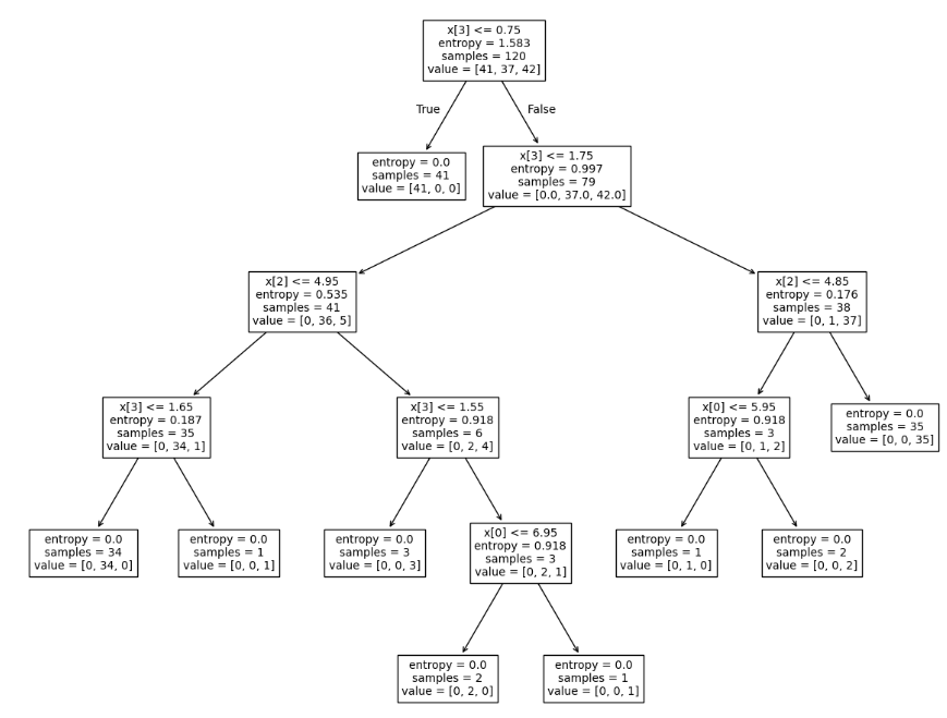
5단계: 예측
# 분류 예측
y_pred =clf.predict(X_test)
print (y_pred)

# 평가: 혼동 행렬 출력
print(confusion_matrix(y_test, y_pred))

# 정확도 출력
print("정확도:", accuracy_score(y_test, y_pred))
[1 1 2 0 1 0 0 0 1 2 1 0 2 1 0 1 2 0 2 1 1 1 1 1 2 0 2 1 2 0]
[[ 9 0 0]
[ 0 13 0]
[ 0 0 8]]
정확도: 1.0
'AI Study > Machine Learning' 카테고리의 다른 글
| SVM: Support Vector Machine (0) | 2025.12.15 |
|---|---|
| K-최근접 이웃: KNN, K-nearest neighbors (0) | 2025.12.15 |
| 연관분석: Apriori Algorithm (0) | 2025.12.15 |
| 군집화, K-Means Clustering (1) | 2025.10.28 |
| 주성분 분석, PCA: Principal Component Analysis (0) | 2025.10.28 |