서포트 벡터 머신
- 지도학습, 분류 및 회귀분석에 유용
- 어느 그룹에 속하는지 판단하는 이진 분류와 다중 분류에 응용
- 선형 또는 비선형 회귀문제에 응용
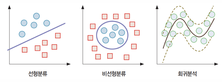
SVM은 클래스를 구분 짓는 거리의 마진(margin)을 최대로 하는 초평면(hyperplane)을 찾고 새로운 개체를 분류하는 방법.


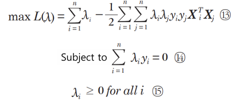
라그랑주 승수법
* 초평면을 구하기 위한 수학
비선형 문제
차원을 늘리면 해결됨. 저차원 To 고차원 매핑함수 φ가 여러개임. Linear, Polynomial 등.


이런식으로 non-linear 문제가 linear problem으로 바뀜.
But φ를 실제로 모든 point에 적용해서 변환하면 메모리와 시간이 엄청나게 들어감.

So, 커널함수를 사용. 우리는 고차원으로 변환한 데이터가 필요한 게 아니라 내적값만 필요함.
(어차피 고차원 변환 후 라그랑주 승수법으로 초평면 뽑을건데, 라그랑주 승수법에서는 내적값만 있으면 됨. 그렇게 최적화 가능)
커널함수 (고차원 매핑함수 φ에 대응하는 커널함수들이 있음)
- Linear
- Poly: polynomial kernel
- RBF: radial basis function kernel
- Sigmoid
실습
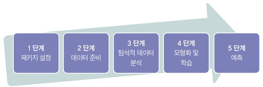
1단계: 패키지 설정
from sklearn import svm
import numpy as np
import matplotlib.pyplot as plt
2단계: 데이터 준비
# 학습용 데이터(기존 개체)
# 입력
X_train = np.array([[2, 3], [1, 2]])
# 라벨
y_train =np.array([1,-1])

# 테스트 데이터
# 입력
X_test = np.array([[3, 3]])
3단계: 탐색적 데이터 분석
#산포도
# 학습용 데이터
plt.scatter(X_train[:, 0], X_train[:, 1],c=y_train)
# 테스트용 데이터
plt.scatter(X_test[:, 0], X_test[:, 1], c='red', marker='D', s=100)
plt.xlabel('x1')
plt.ylabel('x2')
plt.xlim(0,5)
plt.ylim(0,5)
plt.show()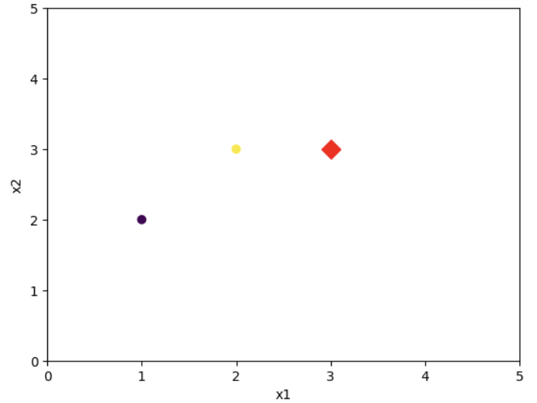
4단계: 모형화 및 학습
# SVM 분류 모형화
clf =svm.SVC(kernel='linear')

# 모형 학습
clf.fit(X_train,y_train)
# 분류별 서포트 벡터의 수
print(clf.n_support_)
# 서포트 벡터
print(clf.support_vectors_)[1 1]
[[1. 2.]
[2. 3.]]
# 서포트 벡터의 색인
print(clf.support_)


# 각 개체들의 색인별 분류
print(clf.classes_)
[1 0]
[-1 1]
# W: 가중치
print(clf.coef_)

# b: 편향
print(clf.intercept_)
[[1. 1.]]
[-4.]
5단계: 예측
# 테스트 데이터의 분류
y_pred = clf.predict(X_test)
print(y_pred)
[1]
유방암 진단 실습
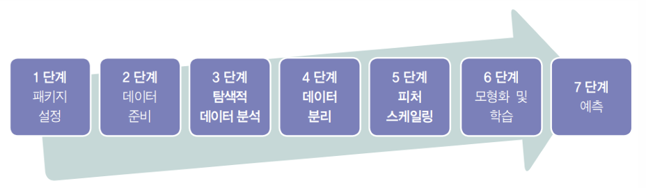
1단계: 패키지 설정
from sklearn.datasets import load_breast_cancer
from sklearn import svm
from sklearn.preprocessing import StandardScaler
from sklearn.model_selection import train_test_split
from sklearn.metrics import confusion_matrix
2단계: 데이터 준비
# 데이터 불러오기
data = load_breast_cancer(as_frame=True)
# 데이터 프레임 출력
print(data.frame) mean radius mean texture mean perimeter mean area mean smoothness \
0 17.99 10.38 122.80 1001.0 0.11840
1 20.57 17.77 132.90 1326.0 0.08474
2 19.69 21.25 130.00 1203.0 0.10960
3 11.42 20.38 77.58 386.1 0.14250
4 20.29 14.34 135.10 1297.0 0.10030
.. ... ... ... ... ...
564 21.56 22.39 142.00 1479.0 0.11100
565 20.13 28.25 131.20 1261.0 0.09780
566 16.60 28.08 108.30 858.1 0.08455
567 20.60 29.33 140.10 1265.0 0.11780
568 7.76 24.54 47.92 181.0 0.05263
mean compactness mean concavity mean concave points mean symmetry \
0 0.27760 0.30010 0.14710 0.2419
1 0.07864 0.08690 0.07017 0.1812
2 0.15990 0.19740 0.12790 0.2069
3 0.28390 0.24140 0.10520 0.2597
4 0.13280 0.19800 0.10430 0.1809
.. ... ... ... ...
564 0.11590 0.24390 0.13890 0.1726
565 0.10340 0.14400 0.09791 0.1752
566 0.10230 0.09251 0.05302 0.1590
567 0.27700 0.35140 0.15200 0.2397
568 0.04362 0.00000 0.00000 0.1587
mean fractal dimension ... worst texture worst perimeter worst area \
0 0.07871 ... 17.33 184.60 2019.0
1 0.05667 ... 23.41 158.80 1956.0
2 0.05999 ... 25.53 152.50 1709.0
3 0.09744 ... 26.50 98.87 567.7
4 0.05883 ... 16.67 152.20 1575.0
.. ... ... ... ... ...
564 0.05623 ... 26.40 166.10 2027.0
565 0.05533 ... 38.25 155.00 1731.0
566 0.05648 ... 34.12 126.70 1124.0
567 0.07016 ... 39.42 184.60 1821.0
568 0.05884 ... 30.37 59.16 268.6
worst smoothness worst compactness worst concavity \
0 0.16220 0.66560 0.7119
1 0.12380 0.18660 0.2416
2 0.14440 0.42450 0.4504
3 0.20980 0.86630 0.6869
4 0.13740 0.20500 0.4000
.. ... ... ...
564 0.14100 0.21130 0.4107
565 0.11660 0.19220 0.3215
566 0.11390 0.30940 0.3403
567 0.16500 0.86810 0.9387
568 0.08996 0.06444 0.0000
worst concave points worst symmetry worst fractal dimension target
0 0.2654 0.4601 0.11890 0
1 0.1860 0.2750 0.08902 0
2 0.2430 0.3613 0.08758 0
3 0.2575 0.6638 0.17300 0
4 0.1625 0.2364 0.07678 0
.. ... ... ... ...
564 0.2216 0.2060 0.07115 0
565 0.1628 0.2572 0.06637 0
566 0.1418 0.2218 0.07820 0
567 0.2650 0.4087 0.12400 0
568 0.0000 0.2871 0.07039 1
[569 rows x 31 columns]
# 입력 부분과 목표 값 출력
print(data.data)
print(data.target)
mean radius mean texture mean perimeter mean area mean smoothness \
0 17.99 10.38 122.80 1001.0 0.11840
1 20.57 17.77 132.90 1326.0 0.08474
2 19.69 21.25 130.00 1203.0 0.10960
3 11.42 20.38 77.58 386.1 0.14250
4 20.29 14.34 135.10 1297.0 0.10030
.. ... ... ... ... ...
564 21.56 22.39 142.00 1479.0 0.11100
565 20.13 28.25 131.20 1261.0 0.09780
566 16.60 28.08 108.30 858.1 0.08455
567 20.60 29.33 140.10 1265.0 0.11780
568 7.76 24.54 47.92 181.0 0.05263
mean compactness mean concavity mean concave points mean symmetry \
0 0.27760 0.30010 0.14710 0.2419
1 0.07864 0.08690 0.07017 0.1812
2 0.15990 0.19740 0.12790 0.2069
3 0.28390 0.24140 0.10520 0.2597
4 0.13280 0.19800 0.10430 0.1809
.. ... ... ... ...
564 0.11590 0.24390 0.13890 0.1726
565 0.10340 0.14400 0.09791 0.1752
566 0.10230 0.09251 0.05302 0.1590
567 0.27700 0.35140 0.15200 0.2397
568 0.04362 0.00000 0.00000 0.1587
mean fractal dimension ... worst radius worst texture \
0 0.07871 ... 25.380 17.33
1 0.05667 ... 24.990 23.41
2 0.05999 ... 23.570 25.53
3 0.09744 ... 14.910 26.50
4 0.05883 ... 22.540 16.67
.. ... ... ... ...
564 0.05623 ... 25.450 26.40
565 0.05533 ... 23.690 38.25
566 0.05648 ... 18.980 34.12
567 0.07016 ... 25.740 39.42
568 0.05884 ... 9.456 30.37
worst perimeter worst area worst smoothness worst compactness \
0 184.60 2019.0 0.16220 0.66560
1 158.80 1956.0 0.12380 0.18660
2 152.50 1709.0 0.14440 0.42450
3 98.87 567.7 0.20980 0.86630
4 152.20 1575.0 0.13740 0.20500
.. ... ... ... ...
564 166.10 2027.0 0.14100 0.21130
565 155.00 1731.0 0.11660 0.19220
566 126.70 1124.0 0.11390 0.30940
567 184.60 1821.0 0.16500 0.86810
568 59.16 268.6 0.08996 0.06444
worst concavity worst concave points worst symmetry \
0 0.7119 0.2654 0.4601
1 0.2416 0.1860 0.2750
2 0.4504 0.2430 0.3613
3 0.6869 0.2575 0.6638
4 0.4000 0.1625 0.2364
.. ... ... ...
564 0.4107 0.2216 0.2060
565 0.3215 0.1628 0.2572
566 0.3403 0.1418 0.2218
567 0.9387 0.2650 0.4087
568 0.0000 0.0000 0.2871
worst fractal dimension
0 0.11890
1 0.08902
2 0.08758
3 0.17300
4 0.07678
.. ...
564 0.07115
565 0.06637
566 0.07820
567 0.12400
568 0.07039
[569 rows x 30 columns]
0 0
1 0
2 0
3 0
4 0
..
564 0
565 0
566 0
567 0
568 1
Name: target, Length: 569, dtype: int64
3단계: 탐색적 데이터 분석
KNN 참고.
4단계: 데이터 분리
# 학습용과 테스트 데이터 분리
X_train,X_test,y_train,y_test=train_test_split(data.data, data.target, test_size=0.3, random_state=1234)

print(X_train.shape)
print(X_test.shape)
print(y_train.shape)
print(y_test.shape)
(398, 30)
(171, 30)
(398,)
(171,)
5단계: 피처 스케일링
# 피처 스케일링: 학습 데이터
scalerX =StandardScaler()
scalerX.fit(X_train)
X_train_std=scalerX.transform(X_train)
print(X_train_std)
[[-1.53753797 -0.55554819 -1.51985982 ... -1.73344373 -0.77142494
0.22129607]
[-0.79609663 -0.38603656 -0.81356785 ... -0.43011095 0.08970515
-0.36303452]
[ 0.21752653 -0.38603656 0.18557689 ... 0.76443594 0.80894448
-0.67502531]
...
[-0.48269225 -0.14686262 -0.46083202 ... -0.21253919 0.1565732
0.16129784]
[ 1.14079887 -0.12364185 1.14739725 ... 0.25197353 0.1679897
-0.23677737]
[-0.41210568 -1.26610378 -0.43253113 ... -0.78299078 -0.89537548
-0.79241315]]
6단계: 모형화 및 학습
# SVM 분류 모형화: 선형분리
clf=svm.SVC(kernel='linear')

# 모형 학습
clf.fit(X_train_std,y_train)
7단계: 예측
# 테스트 데이터의 분류
y_pred=clf.predict(X_test_std)
print(y_pred)
[1 1 1 1 1 1 0 1 0 0 0 1 1 1 1 0 1 1 1 0 1 0 0 0 0 1 0 1 1 1 1 1 0 1 1 1 1
0 1 1 0 1 0 1 1 1 1 1 0 1 1 1 1 0 0 1 1 1 1 0 1 1 1 1 1 0 0 1 1 1 1 0 1 1
1 1 1 0 1 0 1 1 1 0 0 0 0 0 1 0 1 1 1 0 0 1 1 1 1 1 0 0 1 1 0 1 1 0 0 1 0
1 0 0 1 1 1 0 1 0 1 1 1 1 0 1 0 0 1 1 0 1 0 1 1 1 1 1 1 0 1 0 0 1 0 1 1 1
0 1 1 1 0 1 1 0 1 0 0 1 1 1 0 1 1 0 1 1 1 1 0]
# confusion matrix
cf = confusion_matrix(y_test, y_pred)
print(cf)


# 테스트 데이터에 대한 정확도
clf.score(X_test_std, y_test)
[[ 58 8]
[ 1 104]]
0.9473684210526315
'AI Study > Machine Learning' 카테고리의 다른 글
| 의사결정나무: Decision Tree (0) | 2025.12.15 |
|---|---|
| K-최근접 이웃: KNN, K-nearest neighbors (0) | 2025.12.15 |
| 연관분석: Apriori Algorithm (0) | 2025.12.15 |
| 군집화, K-Means Clustering (1) | 2025.10.28 |
| 주성분 분석, PCA: Principal Component Analysis (0) | 2025.10.28 |