분류문제: 새로운 개체와 특성이 가장 가까운 K개의 유사 개체들을 추출하여 빈도가 높은 특정 클래스로 분류.
회귀문제: 유사 개체들의 정량적인 목표 값을 이용하여 하나의 수치적 값을 예측.
[활용 예]
▪ 분류문제
- 새로 가입한 고객은 어떤 그룹에 속할까?
- 새롭게 가입한 회원에게 어떤 영화를 추천할까?
- 저 음악 어떤 장르로 분류할 수 있을까?
▪ 회귀문제
- 고객들의 소득을 파악하면 우리 백화점의 구매금액을 추정할 수 있을까?
- 방의 수와 범죄율을 알면 주택 가격을 추정할 수 있을까?
목표 변수가 범주 변수인 경우: 새로운데이터와 가장 가까운 거리(유사도)에 있는 K개개체들의 다수 분류에 따라 분류.
목표 변수가 양적 변수인 경우: 가장 인접한 K개의 목표 변수의 평균 값으로 하는 회귀문제에 적용.
유사도
- 유클리드 거리 (점과 점 사이의 거리)
- 맨하탄 거리 (격자 형태의 두 지점간 거리)
- 코사인 유사도 (두 벡터 간의 각도)
- 민코브스키 거리 (차수가 1이면 맨하탄 거리, 차수가 2이면 유클리드 거리)

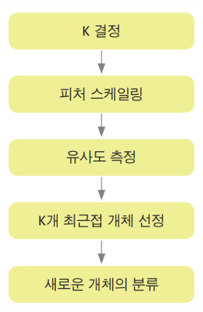
[1] K의 결정.
이진 분류의 경우, 동점을 피하기 위해 K를 홀수로 정함.
최적의 K는 K의 변화에 따른 기존 개체들의 오분류 수를 파악하는 교차검증을 통해 결정.
[2] 피처 스케일링
노멀라이징.
[3] 유사도 측정
표준화된 데이터에서 유사도 측정 함수(유클리드, 코사인 유사도 등)으로 측정
[4] 최근접 이웃 선택
Test 데이터와 raw data와의 유사도가 가장 높은 거로 선택.
실습

분류문제
1 단계: 패키지 설정
from sklearn.neighbors import KNeighborsClassifier
from sklearn.preprocessing import StandardScaler
import numpy as np
import matplotlib.pyplot as plt
2 단계: 데이터 준비
# 학습용 데이터(기존 개체)
# 입력
X_train =np.array([[25, 25],
[33,30],
[38, 30],
[45,35],
[28,40]])
# 라벨
y_train = np.array([0,0,1,1,0])

# 테스트용 데이터(새로운 개체)
# 입력
X_test = np.array([[30, 35]])
3 단계: 탐색적 데이터 분석
# 산포도
# 학습용 데이터
plt.scatter(X_train[:, 0], X_train[:, 1],c=y_train)
# 테스트용 데이터
plt.scatter(X_test[:, 0], X_test[:, 1], c='red', marker='D',s=100)
plt.xlabel('x1')
plt.ylabel('x2')
plt.show()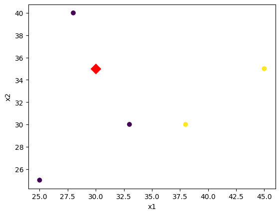
4 단계: 피처 스케일링
# 피처 스케일링: 학습용 데이터
scalerX = StandardScaler()
scalerX.fit(X_train)
X_train_std=scalerX.transform(X_train)
print(X_train_std)
[[-1.23272999 -1.37281295]
[-0.11206636 -0.39223227]
[ 0.58834841 -0.39223227]
[ 1.56892908 0.58834841]
[-0.81248113 1.56892908]]
# 피처 스케일링: 테스트용 데이터
X_test_std= scalerX.transform(X_test)
print(X_test_std)
[[-0.53231522 0.58834841]]
5 단계: 모형화 및 학습
# 모형화
knn = KNeighborsClassifier(n_neighbors = 3, metric='euclidean')
# 학습
knn.fit(X_train_std, y_train)
6 단계: 예측
# 예측
pred = knn.predict(X_test_std)
print(pred)
[0]
# 클래스별 확률 값을 반환
knn.predict_proba(X_test_std)
array([[0.66666667, 0.33333333]])# 인접한 K개의 개체들에 대한 거리와 색인을 반환
dist, index = knn.kneighbors(X_test_std)
print(dist)
print(index)[[1.0198193 1.06683999 1.48910222]]
[[4 1 2]]
회귀문제 (타겟 이 양적 변수)
1 단계: 패키지 설정
from sklearn.neighbors import KNeighborsRegressor
from sklearn.preprocessing import StandardScaler
import numpy as np
import matplotlib.pyplot as plt
2 단계: 데이터 준비
# 학습용 데이터(기존 개체)
# 입력 값
X_train =np.array([[25, 25],
[33,30],
[38,30],
[45,35],
[28,40]])
# 목표 값
y_train = np.array([[10], [20], [30], [40], [50]])

# 테스트용 데이터(새로운 개체)
# 입력
X_test =np.array([[30, 35]])
3 단계: 탐색적 데이터 분석
# 산포도
# 학습용 데이터
plt.scatter(X_train[:, 0], X_train[:,1],c=y_train)
# 테스트용 데이터
plt.scatter(X_test[:, 0], X_test[:,1], c='red', marker='D', s=100)
plt.xlabel('x1')
plt.ylabel('x2')
plt.show()
4 단계: 피처 스케일링
# 피처 스케일링: 학습용 데이터
# 입력 값
scalerX = StandardScaler()
scalerX.fit(X_train)
X_train_std=scalerX.transform(X_train)
print(X_train_std)

# 목표 값
scalerY = StandardScaler()
scalerY.fit(y_train)
y_train_std=scalerY.transform(y_train)
print(y_train_std)
[[-1.23272999 -1.37281295]
[-0.11206636 -0.39223227]
[ 0.58834841 -0.39223227]
[ 1.56892908 0.58834841]
[-0.81248113 1.56892908]]
[[-1.41421356]
[-0.70710678]
[ 0. ]
[ 0.70710678]
[ 1.41421356]]
5 단계: 모형화 및 학습
# 학습

# 모형화
knn = KNeighborsRegressor(n_neighbors = 3, metric='euclidean', weights="uniform")

knn.fit(X_train_std, y_train_std)
6 단계: 예측
# 예측
y_pred = knn.predict(X_test_std)
print(y_pred)


# 예측 값의 역변환
y_pred_inverse = scalerY.inverse_transform(y_pred)
print(y_pred_inverse)
[[0.23570226]]
[[33.33333333]]
유방암 데이터로 실습

1단계: 패키지 설정
from sklearn.datasets import load_breast_cancer
from sklearn.neighbors import KNeighborsClassifier
from sklearn.preprocessing import StandardScaler
from sklearn.model_selection import train_test_split
from sklearn.metrics import confusion_matrix
import pandas as pd
import matplotlib.pyplot as plt
import seaborn as sns
2단계: 데이터 준비
# 데이터 불러오기
data = load_breast_cancer(as_frame=True)

# 데이터 프레임 출력
print(data.frame)
mean radius mean texture mean perimeter mean area mean smoothness \
0 17.99 10.38 122.80 1001.0 0.11840
1 20.57 17.77 132.90 1326.0 0.08474
2 19.69 21.25 130.00 1203.0 0.10960
3 11.42 20.38 77.58 386.1 0.14250
4 20.29 14.34 135.10 1297.0 0.10030
.. ... ... ... ... ...
564 21.56 22.39 142.00 1479.0 0.11100
565 20.13 28.25 131.20 1261.0 0.09780
566 16.60 28.08 108.30 858.1 0.08455
567 20.60 29.33 140.10 1265.0 0.11780
568 7.76 24.54 47.92 181.0 0.05263
mean compactness mean concavity mean concave points mean symmetry \
0 0.27760 0.30010 0.14710 0.2419
1 0.07864 0.08690 0.07017 0.1812
2 0.15990 0.19740 0.12790 0.2069
3 0.28390 0.24140 0.10520 0.2597
4 0.13280 0.19800 0.10430 0.1809
.. ... ... ... ...
564 0.11590 0.24390 0.13890 0.1726
565 0.10340 0.14400 0.09791 0.1752
566 0.10230 0.09251 0.05302 0.1590
567 0.27700 0.35140 0.15200 0.2397
568 0.04362 0.00000 0.00000 0.1587
mean fractal dimension ... worst texture worst perimeter worst area \
0 0.07871 ... 17.33 184.60 2019.0
1 0.05667 ... 23.41 158.80 1956.0
2 0.05999 ... 25.53 152.50 1709.0
3 0.09744 ... 26.50 98.87 567.7
4 0.05883 ... 16.67 152.20 1575.0
.. ... ... ... ... ...
564 0.05623 ... 26.40 166.10 2027.0
565 0.05533 ... 38.25 155.00 1731.0
566 0.05648 ... 34.12 126.70 1124.0
567 0.07016 ... 39.42 184.60 1821.0
568 0.05884 ... 30.37 59.16 268.6
worst smoothness worst compactness worst concavity \
0 0.16220 0.66560 0.7119
1 0.12380 0.18660 0.2416
2 0.14440 0.42450 0.4504
3 0.20980 0.86630 0.6869
4 0.13740 0.20500 0.4000
.. ... ... ...
564 0.14100 0.21130 0.4107
565 0.11660 0.19220 0.3215
566 0.11390 0.30940 0.3403
567 0.16500 0.86810 0.9387
568 0.08996 0.06444 0.0000
worst concave points worst symmetry worst fractal dimension target
0 0.2654 0.4601 0.11890 0
1 0.1860 0.2750 0.08902 0
2 0.2430 0.3613 0.08758 0
3 0.2575 0.6638 0.17300 0
4 0.1625 0.2364 0.07678 0
.. ... ... ... ...
564 0.2216 0.2060 0.07115 0
565 0.1628 0.2572 0.06637 0
566 0.1418 0.2218 0.07820 0
567 0.2650 0.4087 0.12400 0
568 0.0000 0.2871 0.07039 1
[569 rows x 31 columns]
# 입력 부분과 목표 값 출력
print(data.data)
print(data.target)
mean radius mean texture mean perimeter mean area mean smoothness \
0 17.99 10.38 122.80 1001.0 0.11840
1 20.57 17.77 132.90 1326.0 0.08474
2 19.69 21.25 130.00 1203.0 0.10960
3 11.42 20.38 77.58 386.1 0.14250
4 20.29 14.34 135.10 1297.0 0.10030
.. ... ... ... ... ...
564 21.56 22.39 142.00 1479.0 0.11100
565 20.13 28.25 131.20 1261.0 0.09780
566 16.60 28.08 108.30 858.1 0.08455
567 20.60 29.33 140.10 1265.0 0.11780
568 7.76 24.54 47.92 181.0 0.05263
mean compactness mean concavity mean concave points mean symmetry \
0 0.27760 0.30010 0.14710 0.2419
1 0.07864 0.08690 0.07017 0.1812
2 0.15990 0.19740 0.12790 0.2069
3 0.28390 0.24140 0.10520 0.2597
4 0.13280 0.19800 0.10430 0.1809
.. ... ... ... ...
564 0.11590 0.24390 0.13890 0.1726
565 0.10340 0.14400 0.09791 0.1752
566 0.10230 0.09251 0.05302 0.1590
567 0.27700 0.35140 0.15200 0.2397
568 0.04362 0.00000 0.00000 0.1587
mean fractal dimension ... worst radius worst texture \
0 0.07871 ... 25.380 17.33
1 0.05667 ... 24.990 23.41
2 0.05999 ... 23.570 25.53
3 0.09744 ... 14.910 26.50
4 0.05883 ... 22.540 16.67
.. ... ... ... ...
564 0.05623 ... 25.450 26.40
565 0.05533 ... 23.690 38.25
566 0.05648 ... 18.980 34.12
567 0.07016 ... 25.740 39.42
568 0.05884 ... 9.456 30.37
worst perimeter worst area worst smoothness worst compactness \
0 184.60 2019.0 0.16220 0.66560
1 158.80 1956.0 0.12380 0.18660
2 152.50 1709.0 0.14440 0.42450
3 98.87 567.7 0.20980 0.86630
4 152.20 1575.0 0.13740 0.20500
.. ... ... ... ...
564 166.10 2027.0 0.14100 0.21130
565 155.00 1731.0 0.11660 0.19220
566 126.70 1124.0 0.11390 0.30940
567 184.60 1821.0 0.16500 0.86810
568 59.16 268.6 0.08996 0.06444
worst concavity worst concave points worst symmetry \
0 0.7119 0.2654 0.4601
1 0.2416 0.1860 0.2750
2 0.4504 0.2430 0.3613
3 0.6869 0.2575 0.6638
4 0.4000 0.1625 0.2364
.. ... ... ...
564 0.4107 0.2216 0.2060
565 0.3215 0.1628 0.2572
566 0.3403 0.1418 0.2218
567 0.9387 0.2650 0.4087
568 0.0000 0.0000 0.2871
worst fractal dimension
0 0.11890
1 0.08902
2 0.08758
3 0.17300
4 0.07678
.. ...
564 0.07115
565 0.06637
566 0.07820
567 0.12400
568 0.07039
[569 rows x 30 columns]
0 0
1 0
2 0
3 0
4 0
..
564 0
565 0
566 0
567 0
568 1
Name: target, Length: 569, dtype: int64
3단계: 탐색적 데이터 분석
# 데이터 세트 개요
print(data.DESCR)
.. _breast_cancer_dataset:
Breast cancer wisconsin (diagnostic) dataset
--------------------------------------------
**Data Set Characteristics:**
:Number of Instances: 569
:Number of Attributes: 30 numeric, predictive attributes and the class
:Attribute Information:
- radius (mean of distances from center to points on the perimeter)
- texture (standard deviation of gray-scale values)
- perimeter
- area
- smoothness (local variation in radius lengths)
- compactness (perimeter^2 / area - 1.0)
- concavity (severity of concave portions of the contour)
- concave points (number of concave portions of the contour)
- symmetry
- fractal dimension ("coastline approximation" - 1)
The mean, standard error, and "worst" or largest (mean of the three
worst/largest values) of these features were computed for each image,
resulting in 30 features. For instance, field 0 is Mean Radius, field
10 is Radius SE, field 20 is Worst Radius.
- class:
- WDBC-Malignant
- WDBC-Benign
:Summary Statistics:
===================================== ====== ======
Min Max
===================================== ====== ======
radius (mean): 6.981 28.11
texture (mean): 9.71 39.28
perimeter (mean): 43.79 188.5
area (mean): 143.5 2501.0
smoothness (mean): 0.053 0.163
compactness (mean): 0.019 0.345
concavity (mean): 0.0 0.427
concave points (mean): 0.0 0.201
symmetry (mean): 0.106 0.304
fractal dimension (mean): 0.05 0.097
radius (standard error): 0.112 2.873
texture (standard error): 0.36 4.885
perimeter (standard error): 0.757 21.98
area (standard error): 6.802 542.2
smoothness (standard error): 0.002 0.031
compactness (standard error): 0.002 0.135
concavity (standard error): 0.0 0.396
concave points (standard error): 0.0 0.053
symmetry (standard error): 0.008 0.079
fractal dimension (standard error): 0.001 0.03
radius (worst): 7.93 36.04
texture (worst): 12.02 49.54
perimeter (worst): 50.41 251.2
area (worst): 185.2 4254.0
smoothness (worst): 0.071 0.223
compactness (worst): 0.027 1.058
concavity (worst): 0.0 1.252
concave points (worst): 0.0 0.291
symmetry (worst): 0.156 0.664
fractal dimension (worst): 0.055 0.208
===================================== ====== ======
:Missing Attribute Values: None
:Class Distribution: 212 - Malignant, 357 - Benign
:Creator: Dr. William H. Wolberg, W. Nick Street, Olvi L. Mangasarian
:Donor: Nick Street
:Date: November, 1995
This is a copy of UCI ML Breast Cancer Wisconsin (Diagnostic) datasets.
https://goo.gl/U2Uwz2
Features are computed from a digitized image of a fine needle
aspirate (FNA) of a breast mass. They describe
characteristics of the cell nuclei present in the image.
Separating plane described above was obtained using
Multisurface Method-Tree (MSM-T) [K. P. Bennett, "Decision Tree
Construction Via Linear Programming." Proceedings of the 4th
Midwest Artificial Intelligence and Cognitive Science Society,
pp. 97-101, 1992], a classification method which uses linear
programming to construct a decision tree. Relevant features
were selected using an exhaustive search in the space of 1-4
features and 1-3 separating planes.
The actual linear program used to obtain the separating plane
in the 3-dimensional space is that described in:
[K. P. Bennett and O. L. Mangasarian: "Robust Linear
Programming Discrimination of Two Linearly Inseparable Sets",
Optimization Methods and Software 1, 1992, 23-34].
This database is also available through the UW CS ftp server:
ftp ftp.cs.wisc.edu
cd math-prog/cpo-dataset/machine-learn/WDBC/
.. dropdown:: References
- W.N. Street, W.H. Wolberg and O.L. Mangasarian. Nuclear feature extraction
for breast tumor diagnosis. IS&T/SPIE 1993 International Symposium on
Electronic Imaging: Science and Technology, volume 1905, pages 861-870,
San Jose, CA, 1993.
- O.L. Mangasarian, W.N. Street and W.H. Wolberg. Breast cancer diagnosis and
prognosis via linear programming. Operations Research, 43(4), pages 570-577,
July-August 1995.
- W.H. Wolberg, W.N. Street, and O.L. Mangasarian. Machine learning techniques
to diagnose breast cancer from fine-needle aspirates. Cancer Letters 77 (1994)
163-171.
# 데이터 구조 특성 이름과 목표 변수 이름
print(data.feature_names)
print(data.target_names)
['mean radius' 'mean texture' 'mean perimeter' 'mean area'
'mean smoothness' 'mean compactness' 'mean concavity'
'mean concave points' 'mean symmetry' 'mean fractal dimension'
'radius error' 'texture error' 'perimeter error' 'area error'
'smoothness error' 'compactness error' 'concavity error'
'concave points error' 'symmetry error' 'fractal dimension error'
'worst radius' 'worst texture' 'worst perimeter' 'worst area'
'worst smoothness' 'worst compactness' 'worst concavity'
'worst concave points' 'worst symmetry' 'worst fractal dimension']
['malignant' 'benign']
# 변수 간 산포도
data_mean = data.frame[['mean radius','mean texture','mean perimeter','mean area', 'target']]
sns.pairplot(data_mean, hue='target')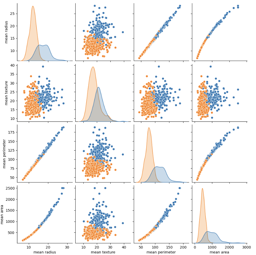
4단계: 데이터 분리
#학습용과 테스트 데이터 분리
X_train,X_test,y_train,y_test=train_test_split(data.data, data.target, test_size=0.3, random_state=1234)
print(X_train.shape)
print(X_test.shape)
print(y_train.shape)
print(y_test.shape)
(398, 30)
(171, 30)
(398,)
(171,)
5단계: 피처 스케일링
# 피처 스케일링: 학습 데이터
scalerX = StandardScaler()
scalerX.fit(X_train)
X_train_std= scalerX.transform(X_train)
print(X_train_std)
[[-1.53753797 -0.55554819 -1.51985982 ... -1.73344373 -0.77142494
0.22129607]
[-0.79609663 -0.38603656 -0.81356785 ... -0.43011095 0.08970515
-0.36303452]
[ 0.21752653 -0.38603656 0.18557689 ... 0.76443594 0.80894448
-0.67502531]
...
[-0.48269225 -0.14686262 -0.46083202 ... -0.21253919 0.1565732
0.16129784]
[ 1.14079887 -0.12364185 1.14739725 ... 0.25197353 0.1679897
-0.23677737]
[-0.41210568 -1.26610378 -0.43253113 ... -0.78299078 -0.89537548
-0.79241315]]
# 피처 스케일링: 테스트 데이터
X_test_std=scalerX.transform(X_test)
print(X_test_std)
[[-0.70856928 0.18287232 -0.70200489 ... -0.5167201 0.46971142
0.26564259]
[-0.95421055 -2.21118915 -0.9661466 ... -1.04371727 -1.35040445
-0.38703381]
[-0.48833918 -0.6553975 -0.38864423 ... 0.27744681 0.51048462
0.99083859]
...
[-0.45163416 -0.19330417 -0.51251192 ... -1.60200162 -0.67356925
-1.04857951]
[-0.45728109 -0.037725 -0.42678891 ... -0.34515008 -1.29984567
-0.65363464]
[ 0.58740016 0.61477866 0.62239509 ... -0.16458949 -0.29682483
-0.25451598]]
6단계: 모형화 및 학습
# 학습용 데이터의 분류 정확도
train_accuracy = []
# 테스트 데이터의 분류 정확도
test_accuracy = []

# 최근접 이웃의 수: 1~15
neighbors = range(1, 16)

for k in neighbors:

  # 모형화
  knn = KNeighborsClassifier(n_neighbors=k)
  # 학습
  knn.fit(X_train_std, y_train)
  # 학습 데이터의 분류 정확도
  score = knn.score(X_train_std, y_train)
  train_accuracy.append(score)
  # 테스트 데이터의 분류 정확도
  score = knn.score(X_test_std, y_test)
  test_accuracy.append(score)

# K의 크기에 따른 분류 정확도 변화
plt.plot(neighbors, train_accuracy, label="train")
plt.plot(neighbors, test_accuracy, label="test")
plt.xlabel("K")
plt.ylabel("Accuracy")
plt.legend()
plt.show()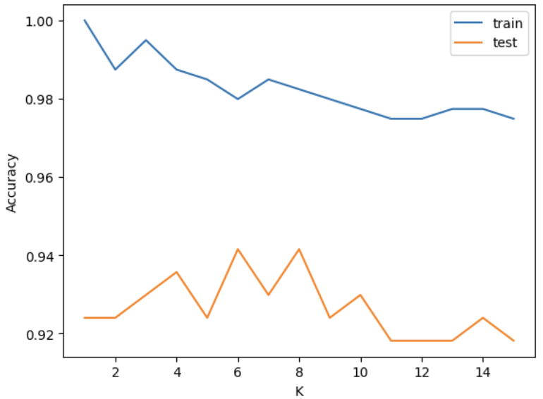
# 테스트 데이터의 분류 정확도
test_accuracy
[0.9239766081871345,
0.9239766081871345,
0.9298245614035088,
0.935672514619883,
0.9239766081871345,
0.9415204678362573,
0.9298245614035088,
0.9415204678362573,
0.9239766081871345,
0.9298245614035088,
0.9181286549707602,
0.9181286549707602,
0.9181286549707602,
0.9239766081871345,
0.9181286549707602]
# 모형화
K= 6
knn = KNeighborsClassifier(n_neighbors=K)
#학습
knn.fit(X_train_std, y_train)
7단계: 예측
# 예측
y_pred = knn.predict(X_test_std)
print(y_pred)
[1 1 1 1 1 1 1 1 0 0 0 1 1 1 1 0 1 1 1 0 1 0 0 0 0 1 0 1 1 1 1 1 0 1 1 1 1
0 1 1 0 1 0 1 1 1 1 1 0 1 1 1 1 0 0 1 1 1 1 0 1 1 1 1 1 0 0 1 1 1 1 0 1 0
1 1 1 0 1 0 1 1 1 1 0 0 0 0 1 1 1 1 1 0 0 1 1 1 1 1 0 0 1 1 0 1 1 0 0 1 0
1 1 0 1 1 1 0 1 0 1 1 1 1 0 1 0 0 1 1 1 1 0 1 1 1 1 1 1 0 1 0 0 1 0 1 0 1
0 1 1 1 0 1 1 0 1 0 0 1 1 1 0 1 1 0 1 1 1 1 0]
# confusion matrix
cf= confusion_matrix(y_test, y_pred)
print (cf)

# 테스트 데이터에 대한 정확도
knn.score(X_test_std, y_test)
[[ 56 10]
[ 0 105]]
0.9415204678362573
'AI Study > Machine Learning' 카테고리의 다른 글
| 의사결정나무: Decision Tree (0) | 2025.12.15 |
|---|---|
| SVM: Support Vector Machine (0) | 2025.12.15 |
| 연관분석: Apriori Algorithm (0) | 2025.12.15 |
| 군집화, K-Means Clustering (1) | 2025.10.28 |
| 주성분 분석, PCA: Principal Component Analysis (0) | 2025.10.28 |